Markowitz’s Mean-Variance Model Derivation in Python

Written by Jiang Rongrong(2019E8010663001)

Interested by “Lecture 3.Quadratic Programing and Portfolio Selection Theory”,I’ve consulted a number of books about Markowitz’s Mean-Variance Model.Therefore,I want to make some discussion about what I’ve learnt and the expeirments when I tried to figure out this model.

Theory Summary

Markowitz made the following assumptions while developing the Mean-Variance Model:

1. Risk of a portfolio is based on the variability of returns from the said portfolio.
2. An investor is risk averse.
3. An investor prefers to increase consumption.
4. The investor’s utility function is concave and increasing, due to his risk aversion and consumption preference.
5. Analysis is based on single period model of investment.
6. An investor either maximizes his portfolio return for a given level of risk or maximizes his return for the minimum risk.
7. An investor is rational in nature.

To choose the best portfolio from a number of possible portfolios, each with different return and risk, two separate decisions are to be made, detailed in the below sections:

1. Determination of a set of efficient portfolios.
2. Selection of the best portfolio out of the efficient set.

Above quotes from wiki

Based on above assumptions and thoughts,Markowitz establish his Mean-Variance Model as follows:

Formula:

Constraints:

notes:x_i stands for the weights of asset i,r_i stands for the return of asset i

Simulations

In this part ,I will try to use random data to simulate the derivation process of Mean-Variance Model.Thanks for my boyfriend’s leading,I choose python as the main tool.And each line of code is with notes if necessary.

First,initiate and import necessary util packages.

Intro of each util package:

• numpy and pandas: Matrix calculate
• matplotlib : Data plot
• cvxopt : A convex solver

import numpy as np
import matplotlib.pyplot as plt
import cvxopt as opt
from cvxopt import blas, solvers
import pandas as pd

np.random.seed(123)

# Turn off progress printing 
solvers.options['show_progress'] = False

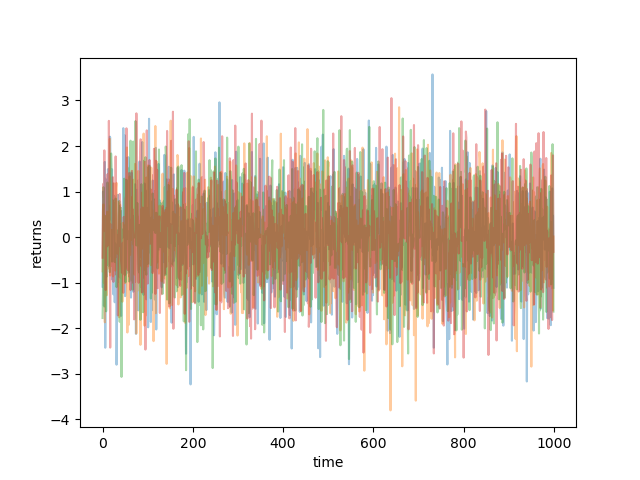
Assume that there are 4 assets, each with a return series of length 1000. The func numpy.random.randn is used to sample returns from a normal distribution.

## NUMBER OF ASSETS
n_assets = 4

## NUMBER OF OBSERVATIONS
n_obs = 1000

return_vec = np.random.randn(n_assets, n_obs)

Plot the return series of the assumed 4 assets.

plt.plot(return_vec.T, alpha=.4);
plt.xlabel('time')
plt.ylabel('returns');

These return series can be used to create a wide range of portfolios. After that random weight vectors and plot those portfolios will be produced. As I want all my capital to be invested, the weights will have to sum to one.

def rand_weights(n):
    ''' Produces n random weights that sum to 1 '''
    k = np.random.rand(n)
    return k / sum(k)

print(rand_weights(n_assets))
print(rand_weights(n_assets))

Next, evaluate how these random portfolios would perform by calculating the mean returns and the volatility (here using standard deviation). I set a filter so that only portfolios with a standard deviation of < 2 are ploted for better illustration.

def random_portfolio(returns):
    ''' 
    Returns the mean and standard deviation of returns for a random portfolio
    '''

    p = np.asmatrix(np.mean(returns, axis=1))
    w = np.asmatrix(rand_weights(returns.shape[0]))
    C = np.asmatrix(np.cov(returns))
        
    mu = w * p.T
    sigma = np.sqrt(w * C * w.T)
    
    # This recursion reduces outliers to keep plots pretty
    if sigma > 2:
        return random_portfolio(returns)
    return mu, sigma

Calculate the return using

R=p^Tw

where R is the expected return, p^T is the transpose of the vector for the mean returns for each time series and w is the weight vector of the portfolio. p is a N*1 column vector, so p^T turns is a 1*N row vector which can be multiplied with the weight (column) vector w to give a scalar result.

Next, Calculate the standard deviation

sigma=sqrt(w^TCw)

where C is the N*N covariance matrix of the returns.

Generate the mean returns and volatility for 500 random portfolios and plot them:

n_portfolios = 500
means, stds = np.column_stack([
    random_portfolio(return_vec) 
    for _ in range(n_portfolios)
])

plt.plot(stds, means, 'o', markersize=5)
plt.xlabel('std')
plt.ylabel('mean')
plt.title('Mean and standard deviation of returns of randomly generated portfolios');

By observing the picture it can be figured out that they form a characteristic parabolic shape called the “Markowitz Bullet” whose upper boundary is called the “efficient frontier”, where investors can have the lowest variance for a given expected return.

Now the efficient frontier in Markowitz-style can be calculated. This is done by minimizing

w^TCw

for fixed expected portfolio return R^Tw while keeping the sum of all the weights equal to 1:

sum(w_i)=1 (i=1,2,3…n)

Here I parametrically run through R^Tw=miu and find the minimum variance for different miu‘s.

def optimal_portfolio(returns):
    n = len(returns)
    returns = np.asmatrix(returns)
    
    N = 100
    mus = [10**(5.0 * t/N - 1.0) for t in range(N)]
    
    # Convert to cvxopt matrices
    S = opt.matrix(np.cov(returns))
    pbar = opt.matrix(np.mean(returns, axis=1))
    
    # Create constraint matrices
    G = -opt.matrix(np.eye(n))   # negative n x n identity matrix
    h = opt.matrix(0.0, (n ,1))
    A = opt.matrix(1.0, (1, n))
    b = opt.matrix(1.0)
    
    # Calculate efficient frontier weights using quadratic programming
    portfolios = [solvers.qp(mu*S, -pbar, G, h, A, b)['x'] 
                  for mu in mus]
    ## CALCULATE RISKS AND RETURNS FOR FRONTIER
    returns = [blas.dot(pbar, x) for x in portfolios]
    risks = [np.sqrt(blas.dot(x, S*x)) for x in portfolios]
    ## CALCULATE THE 2ND DEGREE POLYNOMIAL OF THE FRONTIER CURVE
    m1 = np.polyfit(returns, risks, 2)
    x1 = np.sqrt(m1[2] / m1[0])
    # CALCULATE THE OPTIMAL PORTFOLIO
    wt = solvers.qp(opt.matrix(x1 * S), -pbar, G, h, A, b)['x']
    return np.asarray(wt), returns, risks

weights, returns, risks = optimal_portfolio(return_vec)

plt.plot(stds, means, 'o')
plt.ylabel('mean')
plt.xlabel('std')
plt.plot(risks, returns, 'y-o')
print(weights)

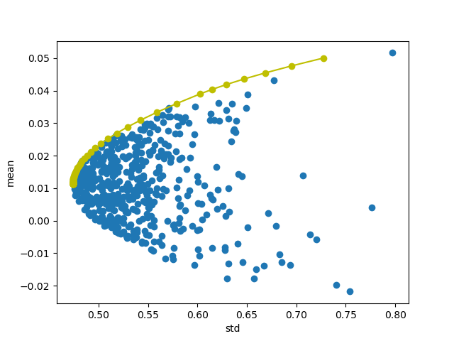
In yellow is the optimal portfolios for each of the desired returns (i.e. the mus). In addition, the weights for one optimal portfolio are also calculated.